5 core models for soft-sensor design

By Eduardo Hernandez, TrendMiner data analytics engineer
Process manufactures hoping to use machine learning to help gather and store operational data may be overwhelmed with the breadth of the discipline. Yet, there are only five common regression algorithms used to create models that become soft sensors, which aid in the collection of time-series data used to analyze process behavior.
There is no right or wrong reason to use one algorithm over another, and no solution will work for a given problem every time. Some statisticians might select a regression model based on experience, while others will use one that best fits a specific process. But there are limitations that must be considered.
The following is a guide to picking a model for soft-sensor design. While the actual selection might be a choice for a data scientist, understanding how a statistician selects a model helps advance collaboration between operations and central data teams.
Understanding soft sensors
Soft sensors can provide information that digital sensors cannot and can offer real-time or almost real-time measurements of critical parameters. Use cases for soft sensors could include staffing shortages, missing sensors, sensor redundancy, or a need for higher-resolution measurements.
Developing a soft sensor can be like other machine-learning projects. Unprocessed and pre-processed time-series and contextual data must be prepared and cleaned. Then, the data scientist must decide if the model will be supervised or unsupervised. Supervised models require a labeled dataset and are more beneficial for creating soft sensors or predictive tags. The final step is to train, test, and deploy the model.
Machine-learning models for soft sensors
The following describes the five most common algorithms for soft sensors and how they might be used by operations.
1. Linear regression
A linear regression produces a function that predicts the value of the target variable (Y ). It does so by creating a function that is a linear combination of one or more manipulated variables (Xs). The formula is:
Y=fX= β1X1+β2X2+…βnXn+C
The weights (βn, also known as the slope if univariate) can be estimated through various techniques; statisticians often use the Least Squares Method (LSM). A data scientist might estimate certain parameters for chemical processes using the linear-regression model because it shows which variable or variables have the most influence on the target. This influence is called feature importance. In some cases, such as estimating the viscosity of a polymer, another machine-learning model must be used because they are too complex for a linear regression.
2. Decision tree
In this model, simple rules from independent variables lead to an approximate value of the target variable. In theory, a decision tree can have as many rules or branches as it needs to fit the data, as shown in Figure 1.
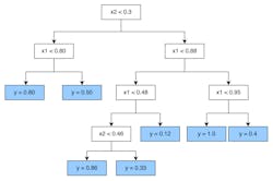
Figure 1: A decision tree model shows rules stemming from other rules in the model.
Overfitting data can be a problem in a decision tree, although it’s not unique to this type of model. Overfitting happens when an algorithm is trained too long. Underfitting, where a model is not trained long enough, also can occur. If either situation happens, the model no longer is useful as a soft sensor.
3. Random forest
A random forest is an extension of the decision tree, but this algorithm combines multiple trees into one model. The combination allows a soft sensor to be more flexible, take on more features, and provide better predictions.
4. Gradient boosting
Much like the random forest, this model combines regression trees, so it is sometimes known as the ensemble model. Unlike a random forest, gradient boosting minimizes the loss function calculated at the end of each tree. Unfortunately, it becomes harder to interpret these models as they grow.
5. Neural network
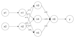
A neural network produces a value for the target variable when it is applied to a regression problem. The most basic is a multiplayer perceptron (MLP). Often, a neural network will have a single input layer and one or more hidden layers (n, each with multiple neutrons). The output layer provides the value.
The weighted inputs of the neurons inside the hidden layer are added and then calculated through an activation function, such as a sigmoid function, which makes the model non-linear. Once the calculation has moved through the hidden layers, it passes a single neuron containing the target variable to the output layer. During training, the selected features and target values are used to determine the appropriate weights that best fit the data, as shown in Figure 3.
Conclusion
Engineers periodically need to collaborate with data scientists on a machine-learning exercise. When they understand the algorithms used during a machine-learning exercise, the contribution from operations greatly improves the time for deployment. Although the data scientist will choose the algorithm that appears to work best, understanding how they apply these models leads to better decisions and a higher level of operational excellence.